
Plotting the FFT of a voltage signal
Published:
Plotting a signal in the frequency domain is a fundamental analysis tool which can provide great insight into the signal’s behaviour. Something I have struggled with in the past is getting the units correct such that the amplitude response of the frequency-domain representation has physical significance. In this blog post I aim to outline how to properly find useful units with which to represent voltage signals.
Testcase
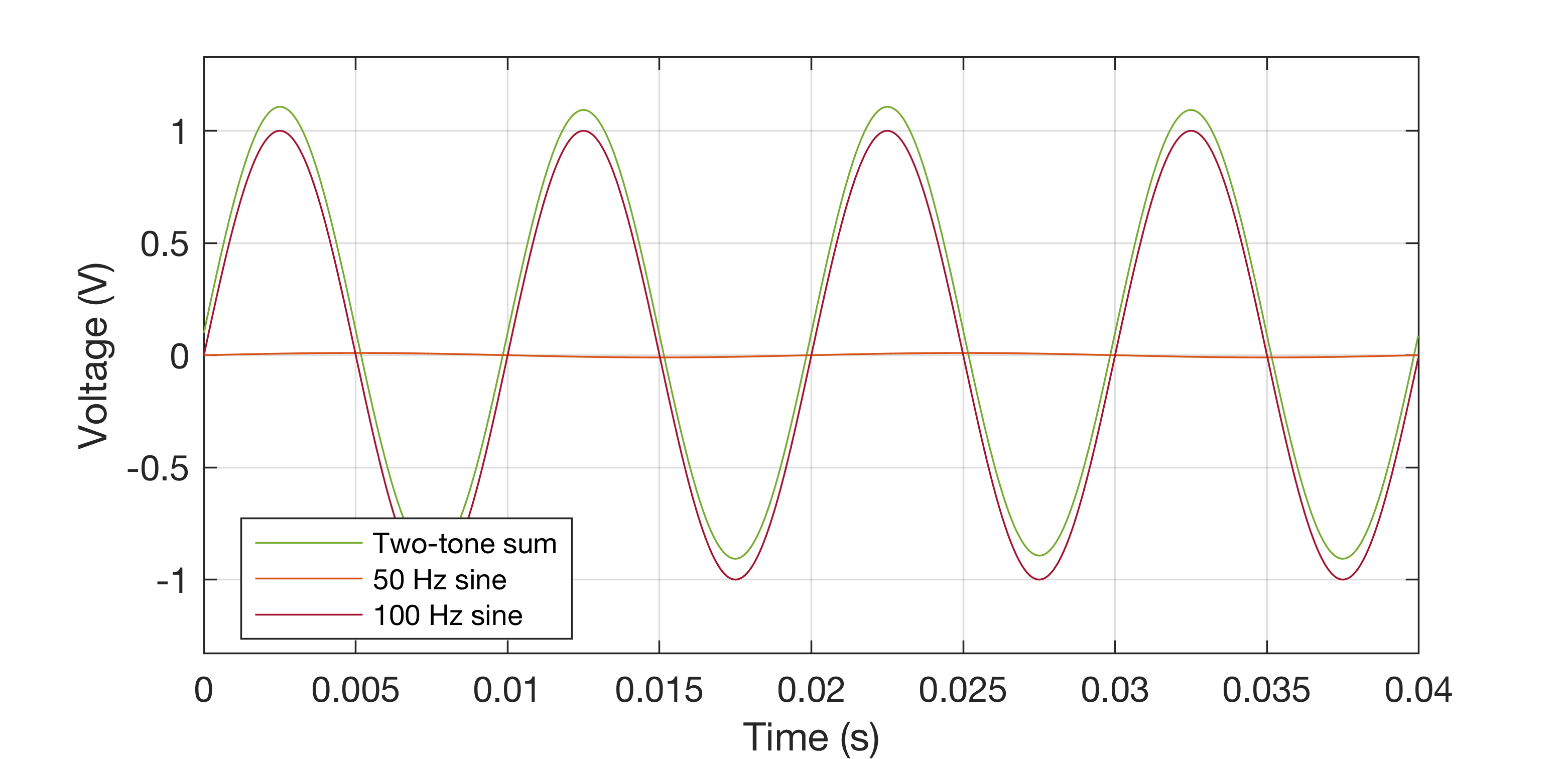
To illustrate the methods in this post, a voltage signal of two sine waves and a DC offset will be used:
| Component | Frequency (Hz) | Peak Voltage (V) |
| 1 | 0 | 0.1 |
| 2 | 50 | 0.01 |
| 3 | 100 | 1 |
The objective is now to provide a method of illustration that enables quick determination of the frequency components in the summed signal and their respective levels.
The DFT
The DFT or Discrete Fourier Transform converts a discrete time-domain signal into a discrete frequency-domain signal. One notable algorithm for calculating the DFT is the the Fast Fourier Transform or FFT which utilises the symmetry of the DFT to optimise performance, and is typically the algorithm implemented by numerical software packages e.g. MATLAB. The DFT algorithm is given by
\[\bar{V}(m) = \sum_{n=0}^{N-1}v(n) \cdot \mathrm{e}^{\frac{-2\pi j}{N} m\cdot n},\quad m=0,\ldots,N-1,\]where \(\bar{V}\) is the DFT of the discrete time domain signal \(v\), each of length \(N\). Immediately there has been a change of units in attempting to find the frequency domain representation: the DFT calculates the sum over the whole length of the signal as opposed to the instantaneous value. This is equivalent to a change from power to energy. Correction is achieved by normalising by the length of the signals i.e.
\[V = \frac{1}{N} \bar{V},\]where \(V\) now is the frequency domain representation of the voltage signal. This is a gotcha which got me as the scaling isn’t included in the implementation in most maths software (specifically MATLAB).
Now, finding the magnitude \(\lvert V \rvert\) already provides a physically significant representation, the results are in the same units as the original signal:
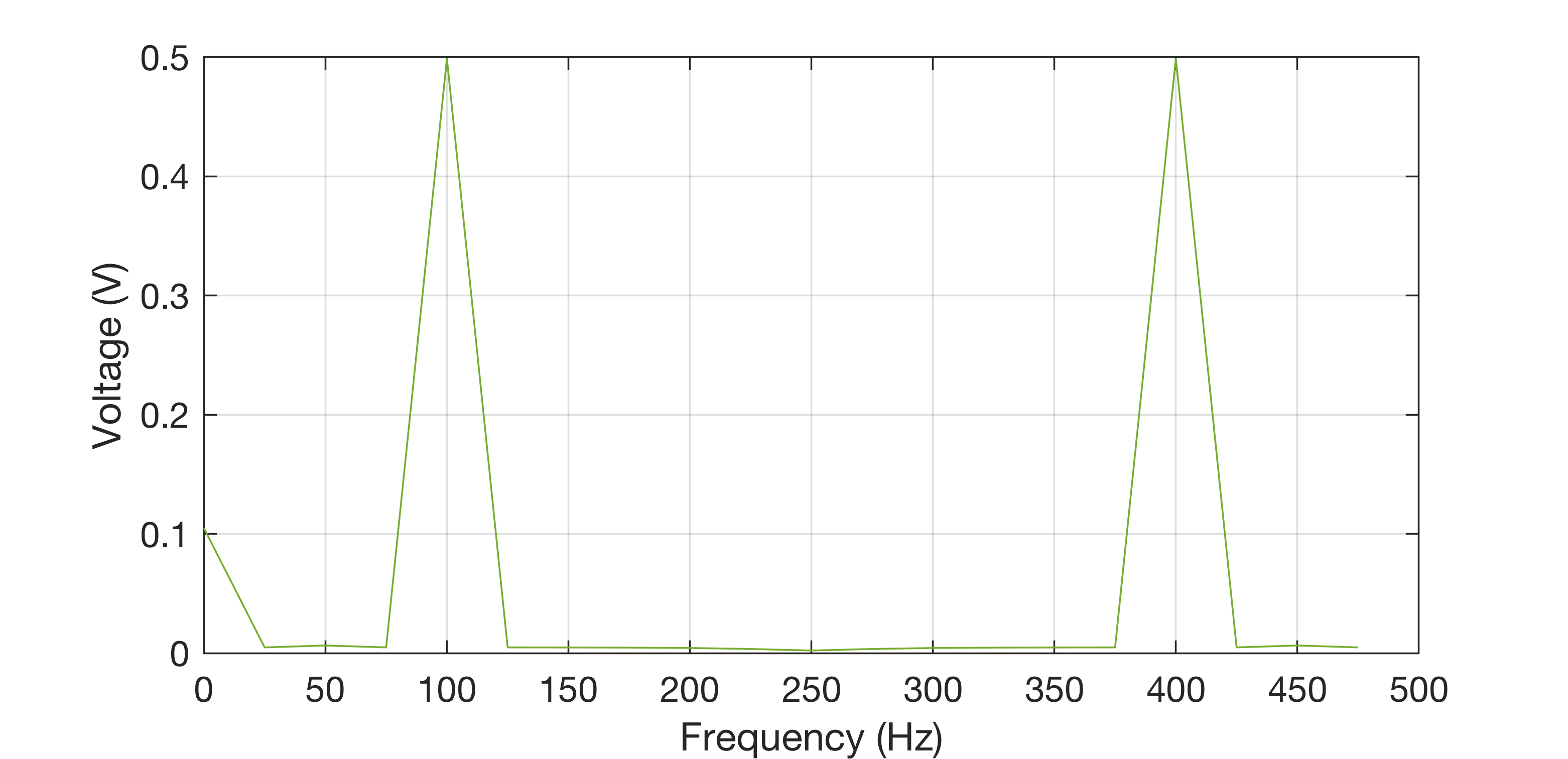
Inspecting the DFT of the signal sampled at \(F_\mathrm{s} = \)500 Hz, the DC component is correct at 0.1 V, although the 100 Hz component is at half the amplitude it should be. This is because the amplitude is split into the bins between 0 Hz - \(F_\mathrm{s}/2\) and \(F_\mathrm{s}/2\) - \(F_\mathrm{s}\) due to the symmetry of the DFT. It is therefore necessary to scale all of the bins that are not DC by a factor of 2:
\[V(m) = \frac{k(m)}{N} \bar{V(m)},\quad\mathrm{where}\quad k(m) = \begin{cases} 2, & m \neq 0\\ 1, & m=0 \end{cases} ,\quad m=0,\ldots,N-1.\]This yields an accurate representation of the signal in the frequency domain. We can do better however as it is difficult to determine the amplitude of the 50 Hz component. This can be solved with…
Decibels
Decibels provide a method of scaling data that is over a large range of values such that it can be read easily, and often helps illustrate trends in data that are otherwise unclear. It is useful here as very small voltages often coincide with very large voltages (typically signals vs noise).
A logarithmic scaling similar to converting to decibels can be achieved using
\[10 \cdot \text{log}_{10}(\lvert V \rvert).\]where the results will now be scaled such that a signal that had a 10 V peak now is at 2 i.e. \(10 \cdot \text{log}_{10}(\lvert 1\times10^2 \rvert) = 2 \), and so a 0.01 V peak is at -2. The exponent in scientific notation is captured in the new value. To present the new data the old values can simply be used as axis labels, and just utilise the new scaling. Most software for plotting encompass a logarithmic plotting option which captures this and displays with the original units, for example with MATLAB and semilogy():
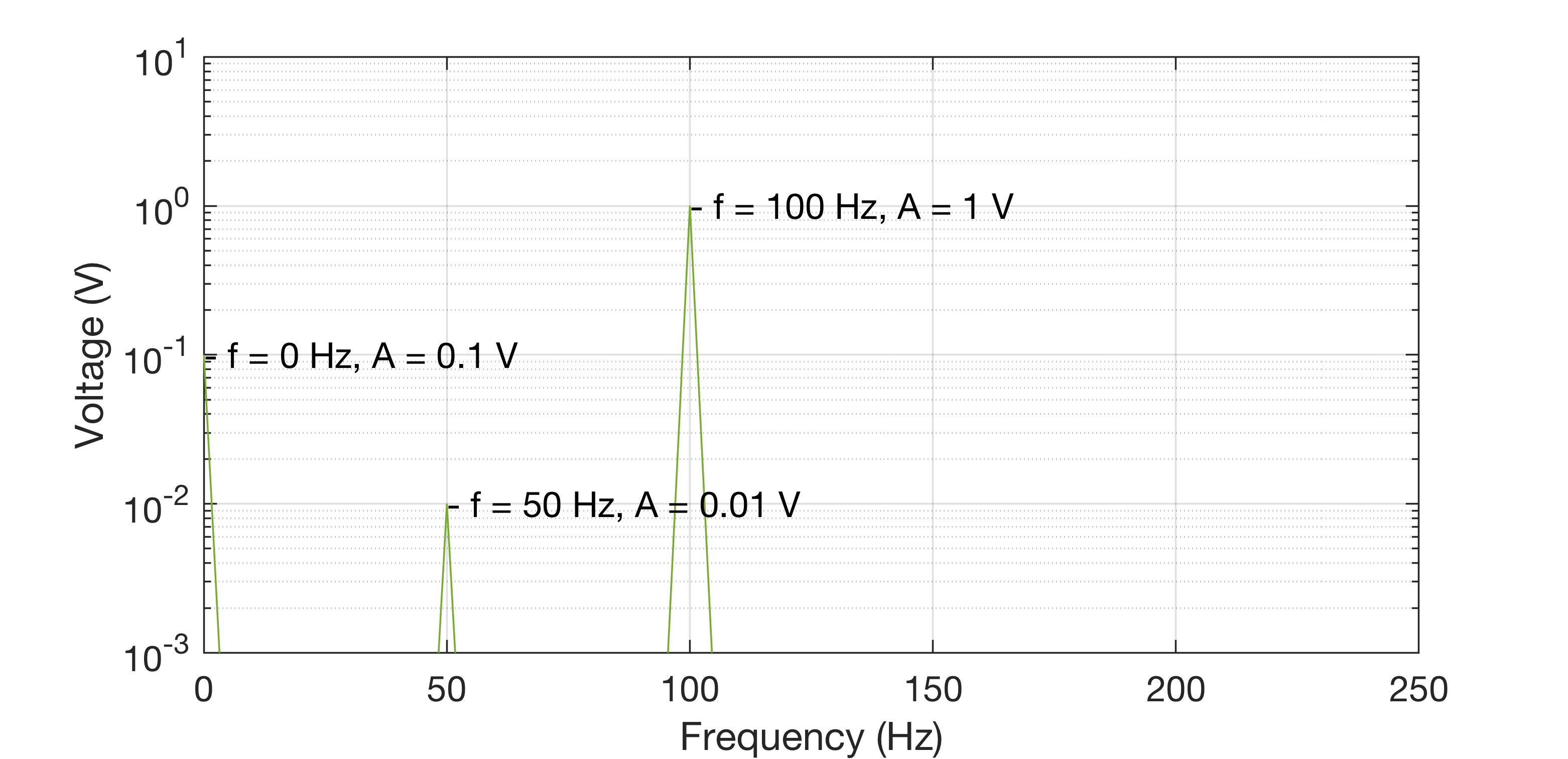
Now the amplitudes are much easier to distinguish over a larger range (the labels help too!).